Notes on Mixture of Experts

These are some notes I took while learning about Mixture of Experts (MoE) architecture. Most of the content is based on the lecture 3 of the Stanford CME295 course on Transformers and LLMs, but I also added some information from other resources. I also discussed about this topic in my podcast, it is in Italian.

Introduction #

Mixture of Experts (MoE) is an architecture that aims to increase the model performance while keeping the inference cost low. This architecture has been used in some recent LLMs such as Mixtral, Qwen and Deepseek but it is now also used in a lot of other models.

Differently from the standard Transformer, you take the original Feed-Forward layer (FFN) and replace it with a sparse version consisting of multiple expert copies. Behind these copies there is a router that selects which of these experts to use for each token in each forward pass at inference time.

Benefits of MoE #

LLMs are huge in terms of number of parameters, this requires a lot of time for both training and inference. The initial idea was to have bigger and bigger models to increase their capabilities. Later a smarter approach, Mixture of Expert (MoE), has been introduced.

MoE allows the model to increase the number of parameters contained in the model, consequently decreasing the loss. At the same time, obviously, this requires more memory to store the parameters. However, the key idea behind MoE is that you can increase the parameters of your models by 10x while limiting the increase in FLOPs. If you have a classic dense model and you increase the number of parameters by 10x, you’ll need to do more computation for each token you process. Instead, with MoE, you can have 10x more parameters but only activate a fraction of them for each token you process. This means having a bigger model while keeping the training cost of a smaller one.

At inference time you have a similar benefit, only a subset of these parameters will be used for each token, keeping the inference cost low. In terms of FLOPS, the MoE model allows to have more parameters per FLOPS compared to a dense model.

Let’s consider Mixtral 8x7B, if you think about the number of parameters, it could be 8*7B = 56B. In reality, the number is lower, 46.7B, because while the FFN layers are multiplied by 8, the rest of the model is shared. Considering what we have said before about the model activations, during the model inference only 2 of the 8 experts are activated. This means that in total, the parameters used for each token are 12.9B, which is the same as a 12B dense model.

Note that even if the number of activate parameters is 12.9B, we still need to load all the parameters 46.7B parameters in the GPU memory.

The other benefit we can have with MoE is the parallelization that we can obtain, each expert can be stored in a different device or GPU. The router will then be responsible for getting the token and activate the correct expert on the correct device. This means that if we have a continuous stream of input data, the different devices can be kept busy and we can have a high throughput. On the contrary, if we have a single device, it might make more sense to directly use a dense model instead of a MoE one, because the cost of loading all the parameters in memory could be higher than the cost of using a smaller dense model.

Where are the experts located? #

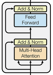
Let’s consider the image above, we have a part of the transformer architecture. Specifically, we are interested in the Feed-Forward layer (FFN). This layer has an amount of parameters that is \( d*d_{ff} + bias \) where \( d \) is the dimension of the input and is O(hundreds) while \( d_{ff} \) is the dimension of the hidden layer and is O(10K). Because of this amount of parameters, the FFN is the best place where to put the MoE architecture. When using MoE you typically replace the FFN with a MoE version of it, where you have trained multiple FFNs and route every token to a different FFN. The router takes the representation of the token and figures out which expert is the best for that token.

Mixture of Experts Architecture #

Given the input \( x \), you ask who should get activated for that input and then you only activate those experts. This is the idea behind Mixture of Experts (MoE) architecture. To do this, not only you need some experts but you also need a gate (or router) that tells you which expert should be involved.

Let’s consider the example in the image above. The gate, we have the input x, the gate G and three experts. The output \( \hat{y} \) can be computed as follows: $$\hat{y} = \sum_{i=1}^{N} g_i(x) \cdot E_i(x)$$

Based on the value that \( g_i(x)$ takes, we can have two different scenarios:

• If \( g_i(x) \) is a binary value, then we have a Sparse MoE. In this case, only the top-k experts will be activated (k is an hyperparameter that we can set) and only a part of the system will be run. If the \( g_i(x) = 0 \) then the corresponding expert won’t be activated. This first solution is used to lower the amount of flops required for inference.
• If instead \( g_i(x) \) is a continuous value between 0 and 1, then we have a Dense MoE. In this case, we do not have a constraint on the number of experts that can be activated. Some weights will be higher than others but all the parameters will be used for all the inputs.

The router \( G \) can be a simple network with a softmax function: $$G(x) = \text{Softmax}(Wx + b)$$ that will give us a probability distribution over the experts.

Inference time #

At inference time, the input x is passed to the Masked Multi-Head Attention (MMHA) and then to the gate G. Even if we have multiple attention heads, the gate is shared across all of them because their inputs are concatenated and projected. The gate then, computes for each token the probability distribution over the experts and selects the top-k experts to activate.

Challenges #

When building LLMs with MoE architecture, we have to face some challenges:

1. Routing collapse: some experts can be more popular than others and can be selected more often by the router while others are never involved in the computation. To mitigate this, a change in the loss can be introduced to force other experts to be selected.

$$\mathcal{L} = \alpha \cdot N \cdot \sum_{i=1}^{N} f_i \cdot P_i$$

Where \( P_i \) is the average probability of selecting the expert \( i \) while \( f_i \) is the fraction of tokens that are routed to expert \( i \).

The key idea behind MoE is that you can increase the parameters of your models while limiting the cost at inference time because you only activate a part of them. The number of experts that you can have is an hyperparameter and is independent of the attention heads. The choice of the expert can be different in the different layers, for instance, we can route token i in layer 1 to expert 1 and in layer 2 to expert 3. The router is layer specific and is trained together with the rest of the model.

Useful resources #

• Stanford CME295 Transformers & LLMs | Autumn 2025 | Lecture 3 - Tranformers & Large Language Models
• Mixtral of experts
• Mixture of Experts Explained